Light Field Image Chroma Upsampling
(This page is under construction, some parts may be missing)

Introduction
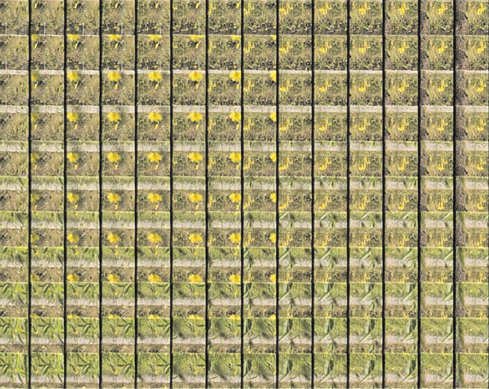
Light Field Image (LFI) is a special kind of image that contains information on the light's direction in the 3D space. In LFI, an image can be seen as an array of many sub-images, each of which is a view of the scene from a different direction. Many applications can be carried out with LFI, such as re-focusing, depth estimation, and 3D reconstruction. However, since LFI is captured by placing a micro-lens array between the main lens and the sensor, the resolution of the LFI is sacrificed. As a result, it became an important issue to enhance the resolution of LFI.
Since our lab has done much research related to chroma upsampling, we decided to also work from this aspect. Moreover, although there is some research on upsampling LFIs, none of them mentioned the part of chroma upsampling. From our perspective, if we can find a way to improve the chroma upsampling method of LFIs, we can probably replace Bayer Filter with another color-filter array to capture more luminance information, and further, enhance the image quality. In this paper, we proposed a CNN-based chroma upsampling method for LFIs, which takes a YUV420 LFI as input and outputs a YUV444 LFI.
Image Compress Pipeline
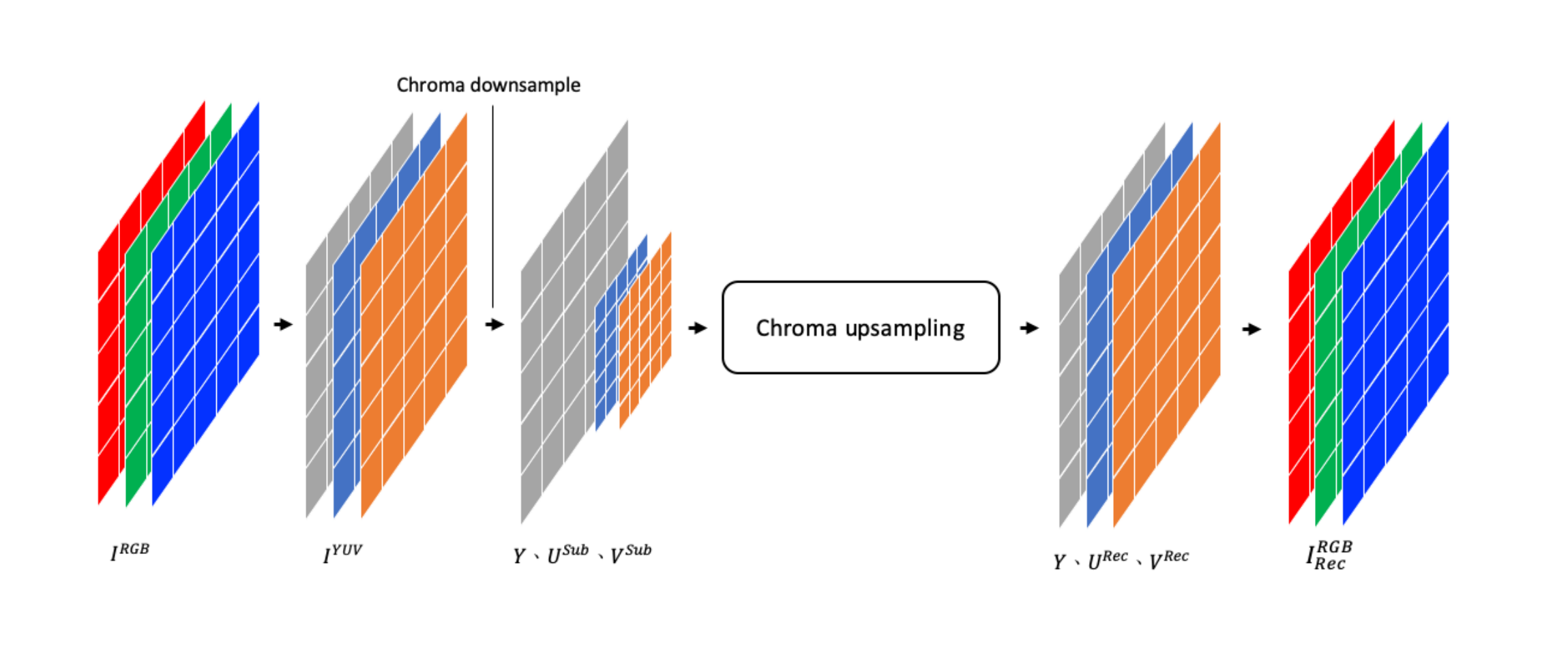
First, I would like to give a brief introduction to the image compress pipeline. Normally, when a computer shows an image on the screen, it uses RGB format to display it. However, since human eyes are more sensitive to luminance than chroma, we can drop some chroma information without losing too much quality. Thus, we can convert RGB into YUV format and subsample the UV channel, where Y and UV store luminance and chroma information, respectively. When we want to display the image, we can simply upsample the UV channel and convert it back to RGB format.

Model
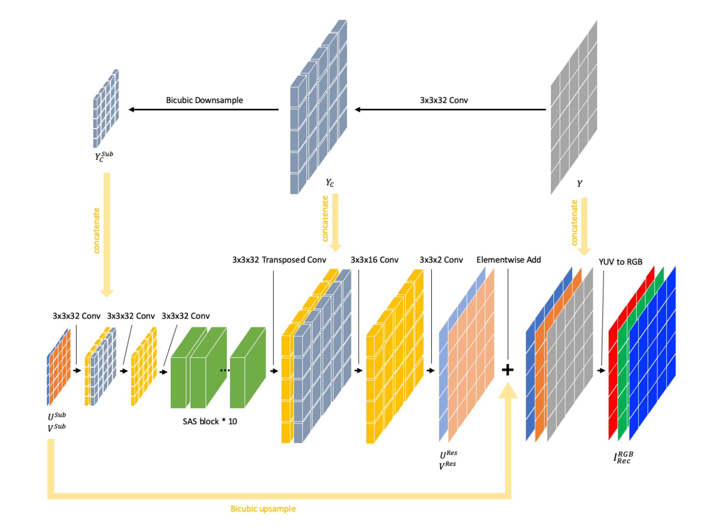
We designed a CNN-based model to perform chroma upsampling. The model takes a YUV420 LFI with 5x5 angular resolution as input and outputs the "residual" of the UV channels, which will be added to the bicubic upsampled UV channel in the end.

(+Model explanation)
The SAS block refers to Spatial-Angular Separable convolution block, in which the convolution is applied to both spatial and angular dimensions. Initially, the axis of a LFI is (Angular X, Angular Y, Spatial X, Spatial Y, channels) and the convolution is applied to the first two dimensions, which is the angular axis. After the convolution, the axis of the LFI is permuted as (spatial X, spatial Y, Angular X, Angular Y, channels) to apply the convolution to the spatial axis.

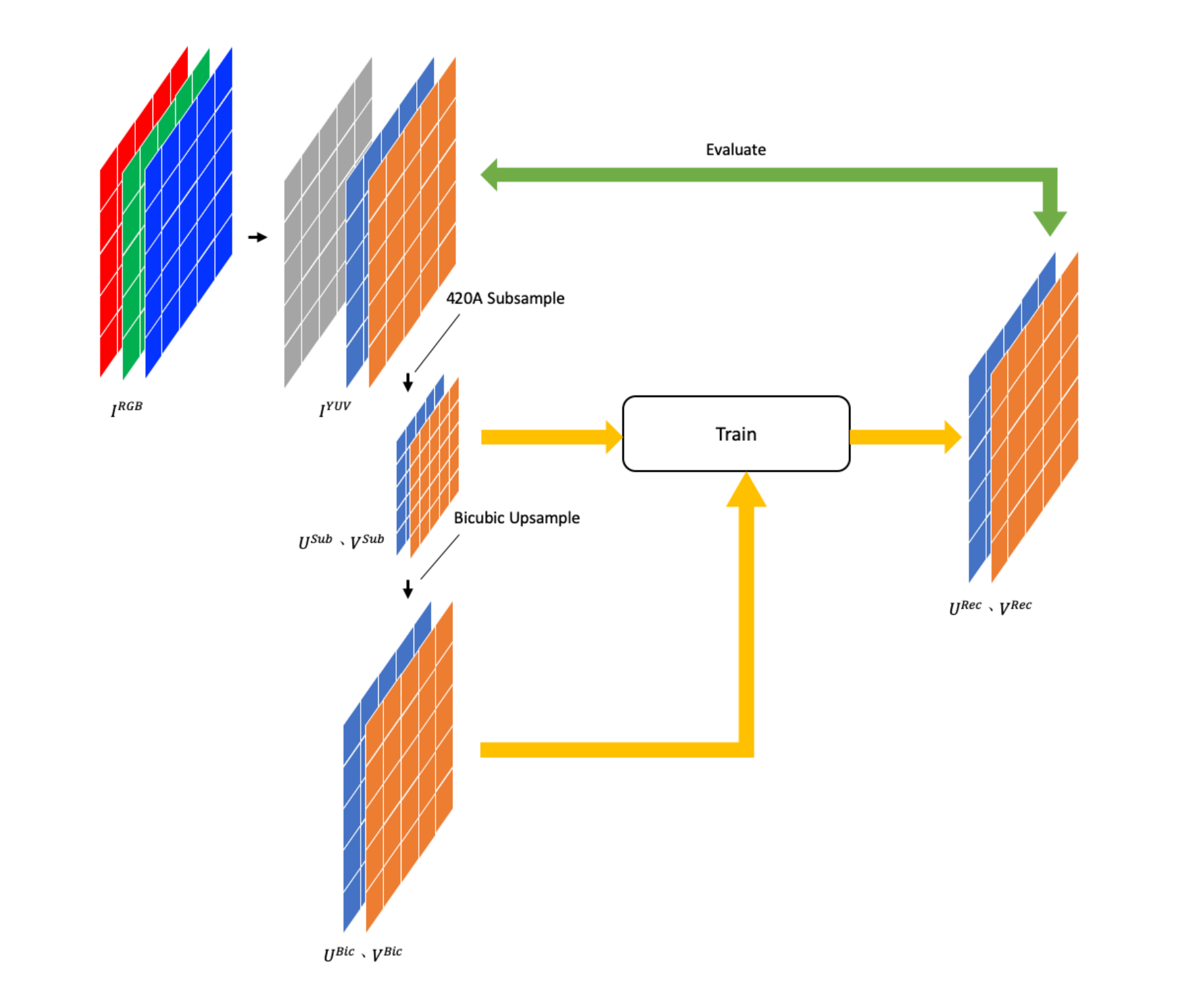
Training Pipeline

Results
Here, we use Peak Signal-to-Noise Ration (PSNR) to evaluate the performance of our model, where the definition of PSNR is as follows:

Since there are no previous research on chroma upsampling of LFIs, we compare our model with the conventional chroma upsampling method, Bicubic and Bilinear. From the results, we can see that our model outperforms the other two methods, with 1.24 dB and 2.22 dB on average.
| #LFI | Proposed | Bicubic | Bilinear |
|---|---|---|---|
| 1 | 43.8130 | 41.9761 | 41.3578 |
| 2 | 42.941 | 40.9295 | 39.0823 |
| 3 | 43.3452 | 42.9033 | 42.0984 |
| 4 | 41.651 | 40.9344 | 39.8863 |
| 5 | 39.0649 | 36.9544 | 34.8554 |
| 6 | 47.9479 | 48.4569 | 49.5385 |
| 7 | 43.5154 | 41.1901 | 40.2849 |
| 8 | 44.3984 | 43.4254 | 41.8508 |
| Average | 43.3346 | 42.0963 | 41.1193 |
Conclusion
Image reference
Cover: http://www.u.arizona.edu/~ppoon/qianpaper.pdf
